A. Non-local modeling for understanding the fracture process and the creation of interface.

We formulate a nonlocal model for calculating the evolution of deformation inside a cracking body. The strain $S(y,x)$ is expressed as a difference quotient of the displacement $u$ resolved along the direction $\mathbf{e}=\frac{y - x}{|y - x|}$, here \begin{equation} \label{strain} S=S(y,x) = \frac{u(y) - u(x)}{|y - x|} \cdot \mathbf{e}. \end{equation}

The acceleration of a material point is now due to the sum of the forces acting on the point from near by points. The constitutive relation relating the strain to force along the direction $\mathbf{e}$ for fixed $x$ and $y$ is initially elastic for small gradients and softens after a critical strain is reached. The nonlocal model treated here and given in (Lipton, 2014) and (Lipton, 2016) is a smooth version of the prototypical microelastic bond (PMB) model introduced by Silling in 2000 (Silling, 2000). The force versus strain relation is illustrated in Figure 1 below.

The length scale of non-local interaction of a point $x$ with its environment is $\epsilon$ and $x$ interacts with all points other points $y$ inside a ball of radius $\epsilon$. The ball centered at $x$ with radius $\epsilon$ is denoted by $\mathcal{H}_\epsilon(x)$.

The stress work density at a material point $x$ is given by \begin{equation} W^\epsilon(x)=\frac{1}{V_\epsilon}\int_{\mathcal{H}_\epsilon(x)} |y-x|\mathcal{W}^\epsilon\big(\mathcal{S},x,y\big)dy \label{eqn-W} \end{equation} where $\mathcal{W}^\epsilon(\mathcal{S},x,y)$ is the force potential per unit length between $x$ and $y$ and $V_\epsilon$ is the area (in 2D) or the volume (in 3D) of the neighborhood $\mathcal{H}_\epsilon(x)$. In this model the force corresponds to the derivitave with respect to strain of a double well potential energy. The potential energy $\mathcal{W}^\epsilon\big(\mathcal{S},x,y\big)$ gives the energy per unit length of a bond at any given strain. Here the elastic well is centered at the origion and the surface energy is the well at infinity.

By Hamilton's principle applied to a bounded body $D\subset\mathbb{R}^d$, $d=2$, $3$, the equation of motion describing the displacement field $u(x,t)$ is \begin{equation} \rho\, u_{tt}(x,t)=\frac{2}{V_\epsilon}\int_{\mathcal{H}_\epsilon(x)\cap D}\, \big(\partial_{\mathcal{S}} \mathcal{W}^\epsilon(\mathcal{S}(y,x)\big)\mathbf{e}\,dy+b(x,t). \label{eqofmotion} \end{equation}

We assume the general form \begin{equation} \mathcal{W}^\epsilon(\mathcal{S},x,y)=\frac{J^\epsilon(|y-x|)}{\epsilon|y-x|} \Psi(|y-x|\mathcal{S}^2) \label{eqn-WJPsi} \end{equation} where $J^\epsilon(|y-x|)=J(|y-x|/\epsilon)>0$ is a weight function and $\Psi:[0,\infty)\rightarrow\mathbb{R}^+$ is a continuously differentiable function such that $\Psi(0)=0$, $\Psi'(0)>0$, and $ \Psi_\infty:=\lim_{r\rightarrow \infty}\Psi(r) < \infty$. The pairwise force density is then given by \begin{equation} \partial_\mathcal{S}\mathcal{W}^\epsilon(\mathcal{S},x,y)= \frac{2J^\epsilon(|y-x|)}{\epsilon}\Psi'\big(|y-x|\{\mathcal{S}^2\big)\mathcal{S}. \label{force} \end{equation} For fixed $x$ and $y$, there is a unique maximum in the curve of force versus strain, see Figure 1. The location of this maximum can depend on the distance between $x$ and $y$ and occurs at the strain $\mathcal{S}_c$ such that $\partial^2\mathcal{W}^\epsilon/\partial\mathcal{S}^2(\mathcal{S}_c,y-x)=0$. This value is $\mathcal{S}_c=\mathcal{S}_c(x,y):=\sqrt{\overline{r}/|y-x|}$, where $\overline{r}$ is the unique number such that $\Psi'(\overline{r})+2\overline{r}\Psi''(\overline{r})=0$. The evolution equation for the displacement inside the body is complemented by bounded initial conditions for the displacement $u_0\in L^2(D;\mathbb{R}^d)$ and velocity ${v}_0\in L^2(D;\mathbb{R}^d)$. One easily finds that the problem admits a unique evolution $ u(x,t)$ in $C^2([0,T];L^2(D;\mathbb{R}^d))$. Direct calculation shows that energy balance holds at each instant of the evolution, see (Lipton, 2014), (Lipton, 2016). The dynamics given by \ref{eqofmotion} is called cohesive dynamcs based on the cohesive nature of the force strain relation.

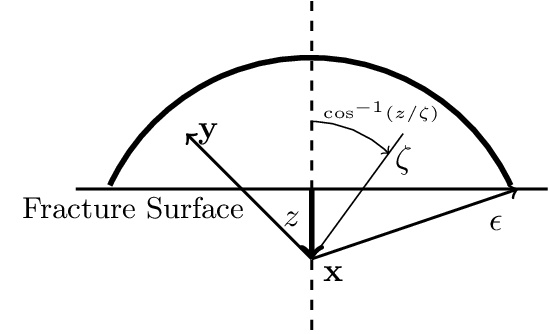
For finite horizon $\epsilon>0$ the elastic moduli and critical energy release rate are recovered directly from the strain potential $\mathcal{W}^\epsilon(\mathcal{S},x,y)$. First suppose the displacement inside $\mathcal{H}_\epsilon(x)$ is affine, that is, $u(x)=Fx$ where $F$ is a constant matrix. For small strains, i.e., $\mathcal{S}=Fe\cdot e\ll\mathcal{S}_c$, the strain potential is linear elastic to leading order and characterized by elastic moduli $\mu$ and $\lambda$ associated with a linear elastic isotropic material \begin{eqnarray} W(x)&=&\frac{1}{V_\epsilon}\int_{H_\epsilon(x)}|y-x|\mathcal{W}^\epsilon(\mathcal{S}(x,y)\,dy\nonumber\\ &=&\mu |F|^2+\frac{\lambda}{2} |Tr\{F\}|^2+O(\epsilon|F|^4). \label{LEFMequality} \end{eqnarray} The elastic moduli $\lambda$ and $\mu$ are calculated directly from the strain energy density and are given by \begin{equation}\label{calibrate1} \mu=\lambda=M\frac{1}{d+2} \Psi'(0) \,, \end{equation} where the constant $M=\int_{0}^1r^{d}J(r)dr$ for dimensions $d=2,3$. In regions of discontinuity the same strain potential is used to calculate the amount of energy consumed by a crack per unit area of crack growth, i.e., the critical energy release rate $\mathcal{G}$. Calculation shows that $\mathcal{G}_c$ equals the work necessary to eliminate force interaction on either side of a fracture surface per unit fracture area and is given in three dimensions by \begin{equation} \mathcal{G}_c=\frac{4\pi}{V_d}\int_0^\epsilon\int_z^\epsilon\int_0^{\cos^{-1}(z/\zeta)} \mathcal{W}^\epsilon(\infty,\zeta)\zeta^2\sin{\phi}\,d\phi\,d\zeta\,dz \label{calibrate2formula} \end{equation} where $\zeta=|y-x|$ and $V_d$ is the volume of the $d$ dimensional unit ball, see Figure 2. In $d$ dimensions, the result is \begin{equation} \mathcal{G}_c=M\frac{2\omega_{d-1}}{\omega_d}\, \Psi_\infty\,, \label{calibrate2formulad} \end{equation} where $\omega_{d}$ is the volume of the $d$ dimensional unit ball, $\omega_1=2,\omega_2=\pi,\omega_3=4\pi/3$.

It is crucial to note that $\mathcal{G}_c$ is independent of the length scale of nonlocal interaction. This is due to our choice of scaling by $\epsilon^{-1}$ in our formulation of the energy.

We prescribe a bounded initial displacement field $u_0(x)$ and bounded initial velocity field ${v}_0(x)$ with bounded Griffith fracture energy given by \begin{eqnarray} \int_{D}\,\mu |\mathcal{E} u_0|^2+\frac{\lambda}{2} |{\rm div}\, u_0|^2\,dx+\mathcal{G}|\mathcal{J}_{u_0}|\leq C \label{LEFMboundinitil} \end{eqnarray} for some $C<\infty$. Here $\mathcal{J}_{u_0}$ is the initial crack set across which the displacement $u_0$ has a jump discontinuity. This jump set need not be geometrically simple; it can be a complex network of cracks. $|\mathcal{J}_{u_0}|=H^{d-1}(J_{u_0})$ is the $d-1$ dimensional Hausdorff measure of the jump set. This agrees with the total surface area (length) of the crack network for sufficently regular cracks for $d=3(2)$. The strain tensor associated with the initial displacement $u_0$ is denoted by $\mathcal{E} u_0$. Consider the sequence of solutions $u^{\epsilon}$ of the initial value problem associated with progressively smaller peridynamic horizons $\epsilon$. The peridynamic evolutions $u^{\epsilon}$ converge in mean square uniformly in time to a limit evolution $u^0(x,t)$ in $C([0,T];L_0^2(D,\mathbb{R}^d )$ and $u_t^0(x,t)$ in $L^2([0,T]\times D;\mathbb{R}^{d})$ with the same initial data, i.e., \begin{eqnarray} \lim_{\epsilon\rightarrow 0}\max_{0\leq t\leq T}\int_D|u^{\epsilon}(x,t)-u^0(x,t)|^2\,dx=0, \label{unifconvg} \end{eqnarray} see (Lipton, 2014) and (Lipton, 2016). It is found that the limit evolution $u^0(x,t)$ has bounded Griffith surface energy and elastic energy given by \begin{eqnarray} \int_{D}\,\mu |\mathcal{E} u^0(t)|^2+\frac{\lambda}{2} |{\rm div}\,u^0(t)|^2\,dx+\mathcal{G}|\mathcal{J}_{u^0(t)}|\leq C, \label{LEFMbound} \end{eqnarray} for $0\leq t\leq T$, where $\mathcal{J}_{u^0(t)}$ denotes the evolving fracture surface inside the domain $D$, (Lipton, 2014), (Lipton, 2016). The limit evolution $u^0(t)$ is found to lie in the space of special functions of bounded deformation SBD, see (Lipton, 2016). For functions in SBD the strain $\mathcal{S}(x,y)$ is related to the strain tensor $\mathcal{E}u$ by \begin{equation} \lim_{\epsilon\rightarrow 0}\frac{1}{V_\epsilon}\int_{\mathcal{H}_\epsilon(x)}|\mathcal{S}-\mathcal{E}u(x) e\cdot e|\,dy, \label{equatesandE} \end{equation} for almost every $x$ in $D$. The jump set $\mathcal{J}_{u^0(t)}$ is the countable union of rectifiable surfaces (arcs) for $d=3(2)$, see (Ambrosio, Coscia, and Dal Maso, 1997).

In domains away from the crack set the limit evolution satisfies local linear elastodynamics (the PDEs of the standard theory of solid mechanics). Fix a tolerance $\tau>0$. If for subdomains $D'\subset D$ and for times $0\leq t\leq T $ the associated strains $\mathcal{S}_{u^\epsilon}$ satisfy $|\mathcal{S}_{u^\epsilon}|\leq S_c$ for every $\epsilon<\tau$ then it is found that the limit evolution $u^0(t,x)$ is governed by the PDE \begin{eqnarray} \rho u^0_{tt}(t,x)= {\rm div}\sigma(t,x)+b(t,x), \hbox{on $[0,T]\times D'$}, \label{waveequationn} \end{eqnarray} where the stress tensor $\sigma$ is given by \begin{eqnarray} \sigma =\lambda I_d Tr(\mathcal{E}\,u^0)+2\mu \mathcal{E}u^0, \label{stress} \end{eqnarray} $I_d$ is the identity on $\mathbb{R}^d$, and $Tr(\mathcal{E}\,u^0)$ is the trace of the strain. To summarize in the limit of small horizon $\epsilon\rightarrow 0$ peridynamic solutions converge in mean square to limit solutions that are linear elastodynamic away from the crack set, that is, the PDEs of the local theory hold at points off of the crack. The elastodynamic balance laws are characterized by elastic moduli $\mu$, $\lambda$. The evolving crack set possesses bounded Griffith surface free energy associated with the critical energy release rate $\mathcal{G}_c$. These convergence and localization results are established in the papers (Lipton, 2014), (Lipton, 2016).

The strategy for proving (\ref{unifconvg}) and (\ref{LEFMbound}) consists of five steps:

1. Constructing upper bounds on the kinetic and potential energy of the evolutions that hold uniformly for $0\leq t\leq T$ and $0<\epsilon$.
2. Showing compactness of the evolution $u^\epsilon(t)$ in $L^2(D)$ for each time $0\leq t\leq T$.
3. Showing uniform Lipschitz continuity in time with respect to $\epsilon$ via the Gronwall inequality.
4. Showing limit points of the sequence $\{u^\epsilon(t)\}$ belong to $SBD$ for each time $0\leq t\leq T$.
5. Point wise convergence of the nonlocal potential energies to the Griffith fracture energy using the SBD structure theorem (Ambrosio, Coscia, and Dal Maso, 1997).

In the next section the kinetic relations for evolution of the crack tip in the limit of vanishing non locality is described, see (Jha and Lipton, 2020). It is found to be given precisly by the well known kinetic relations for Linear Elastic Fracture Mechanics, (Freund 1989), (Ravi-Chandar 2004), (Anderson 1994).

B. Kinetic relations for Linear Elastic Fracture Mechanics implicitly defined by the double well peridynamic model

The well known kinetic relation for the velocity of the crack tip, (Freund 1989), (Ravi-Chandar 2004), (Anderson 1994), follows from the nonlocal model in the limit of vanishing horizon. This is established in (Jha and Lipton, 2020) and described below.

The kinetic relation of LEFM is recovered from the nonlocal model noting that the same nonlocal equation of motion applies everywhere in the body (Jha and Lipton, 2020). In this project we have established the following principle for the nonlocal model:

Local power balance is given by the stationarity in time of the internal energy of a small domain containing the crack tip.

As expected Mott's hypothesis is no longer needed as the crack and intact material are described by one and the same model. This is seen through a novel approach to calculate the time rate of change of internal energy. The change in internal energy is shown to be the difference between the elastic energy flowing into the crack and the kinetic energy and stress work flux flowing into the domain. To leading order the stress work flux is precisely the rate of energy needed to create new surface. These results are obtained directly and exclusively from the dynamics governed by the nonlocal Cauchy equations of motion for a continuum body. This is the explicit connection between the nonlocal Cauchy equations of motion derived from double well potentials (cohesive dynamics) and the energy rate required to make new surface. For remote boundary loading we apply energy balance and pass to the local limit in the nonlocal dynamics to recover the celebrated kinetic relation for the modern theory of dynamic fracture mechanics articulated in (Freund 1989), (Ravi-Chandar 2004), (Anderson 1994).

The principal point of peridynamic modeling is that crack motion is part of the solution and emerges from the nonlocal dynamics. This is the hallmark of peridynamic modeling (Silling 2000), (Ha and Bobaru 2010). Therefore, as we have shown (Jha and Lipton, 2020), the kinetic relations for crack motion follow directly from cohesive dynamics. A numerical simulation is presented below that shows a crack moving at constant speed satisfying energy balance at the crack tip. This simulation is given in (Jha and Lipton, 2020). The numerical computation also shows that the stress work flux is nearly equal to the energy release rate as anticipated by the theory.

Fig. 3

Before introducing the numerical simulation the crack is described in the context of nonlocal modeling. In this context the crack is considered a zone of material failure. To fix ideas consider a thin precracked specimen of fixed length and width and height centered along the $x_2=0$ axis. It is being pulled apart by equal and oppositly directed layers of body force on the top and bottom faces of the specimen. It is characterized by the failure zone centerline. The failure zone centerline starts at the prescrack on the lefthand side of the specimen and propagates twards the right into the interior of the specimen. The force between two points $x$ and $y$ separated by the failure zone centerline is zero. The failure zone is symmetric about the center line and is the grey region in the figure above. For the boundary conditions chosen here failure is in tension and confined to a neighborhood of the $x_2=0$ axis of width $2\epsilon$. Just in front of the failure zone is the process zone where the force between two points $x$ and $y$ on either side of the $x_2=0$ axis is decreasing with increasing strain. At the leading edge of the crack one sees force softening between points $x$ and $y$ and as the crack centerline moves forward passing between $x$ and $y$ the force between $x$ and $y$ decreases to zero. It needs to be stressed the failure zone and process zone emerge from the nonlocal dynamics and are not prescribed. For example see figure 7.

Consider a sample of material with Young's modulus $E = 88$ kPa, Poisson's ratio $\nu = 0.25$, and material density $\rho = 1011.2$ kg/$\text{m}^3$. The Rayleigh wave speed and shear wave speed for the sample are $c_R = 5.502$ m/s and $c_s = 5.9$ m/s respectively. The numerical simulation using these values of $\nu$, $\rho$, $c_R$, and $c_s$ is motivated by the experiments carried out in (Goldman, et al. 2010) and the material domain, horizon, discretization, and boundary conditions are described in figure 5. In this work we assume plane stress conditions. We consider a pre-cracked specimen as shown in figure 5. The pre-crack is of length $l = 3$ mm. The critical energy release rate is taken to be $\mathcal{G}_c = 20$ J/$\text{m}^2$. The force potential is $\Psi(r^2) = c (1-\exp[-\beta r^2])$, where $c,\beta$ are constants. The influence function is of the form $J(r) = 1 - r$. Equations \eqref{calibrate1} and \eqref{calibrate2formulad} are used to calibrate the values of the parameters $c,\beta$. For the material properties listed above we get $c = 15.705$, $\beta = 8965.378$. We define the damage $Z(x)$ at a material point $x$ as follows: \begin{align} Z(x) = \sup_{y \in \mathcal{H}_{\epsilon}({x})} \frac{|S(y, x, u(t))|}{S_c(y, x)}. \end{align} A value $Z > 1$ implies that there are neighboring points $y$ for which the bond-strain between points $y$ and $x$ lies above the critical strain. Here the union of the failure zone and process zone correspond to the set of points where $Z>1$.

Fig. 4

We consider a small region $\mathcal{P}_\delta(t)$ of diameter $\delta$ containing the crack tip and moving with it at $V^\epsilon$ as it travels from the notch to the interior of the specimen, see the figure above. Here the boundary of $\mathcal{P}_\delta(t)$ is denoted by $\Gamma_\delta(t)$. This domain contains undamaged material surrounding the crack as well as the crack itself described by the failure zone. This is in distinct contrast to the $J$ integral formulations where the crack is assumed infinitesimally thin and the region surrounding the crack tip does not include the crack.

Recall the kinetic energy density is given by $T^\epsilon=\rho|\dot u^\epsilon(x,t)|^2/2$ and the stress work density for the nonlocal model given by $W^\epsilon(x)=\int_{\mathcal{H}_\epsilon(x)}|y-x|\mathcal{W}^\epsilon (S(y,x,u^\epsilon(t)))\,dy$. The rate of elastic energy flowing into $\mathcal{P}_\delta(t)$ through its boundary $\Gamma_\delta(t)$ is denoted by $E^\epsilon(\Gamma_\delta)$ and the total rate of change of internal energy inside $\mathcal{P}_\delta(t)$ is $$ \frac{d}{dt}\int_{\mathcal{P}_\delta}T^\epsilon+ W^\epsilon dx.$$

The plot of crack velocity and deformation field surrounding the crack tip centerline at three selected times are shown in figure 6. Damage in the reference configuration is plotted in figure 7. The figure shows that damage is localized and corresponds to the crack in the nonlocal model and is of width $2(\epsilon+h)$. Here $h$ denotes the discretization length scale and $\epsilon$ the horizon length scale and $h$ is taken to be significantly smaller than $\epsilon$. The crack velocity history given by figure 6 is in qualitative agreement with experimental results (Goldman, et al. 2010). There is an initial increase in crack speed, but as waves reflect back from the boundary onto the crack tip the velocity becomes roughly constant. To display the crack opening displacement and the deformation of the specimen we have added the displacement field at the node to its nodal location. This is done for all nodal points in the specimen.

Next, we focus on the regime of near constant crack speed corresponding to the time interval $[0.9647, 0.9801]$. Before presenting the results, we introduce the notation used in the subsequent figures \begin{align}\label{eq:plot_labels} WV &:= \int_{\Gamma_\delta} W^\epsilon V^\epsilon \cdot n ds, \notag \\ {F}_{pd} &:=- E^\epsilon(\Gamma_\delta) \notag \\ \dot{E} &:= \frac{d}{dt}\int_{\mathcal{P}_\delta}T^\epsilon+ W^\epsilon dx, \end{align} where $V^\epsilon$ is the crack velocity. For the material with the critical energy release rate $G_c$, $G_c V^\epsilon$ is the required rate of energy to advance the crack. All plotted quantities are in units of Joules/s.

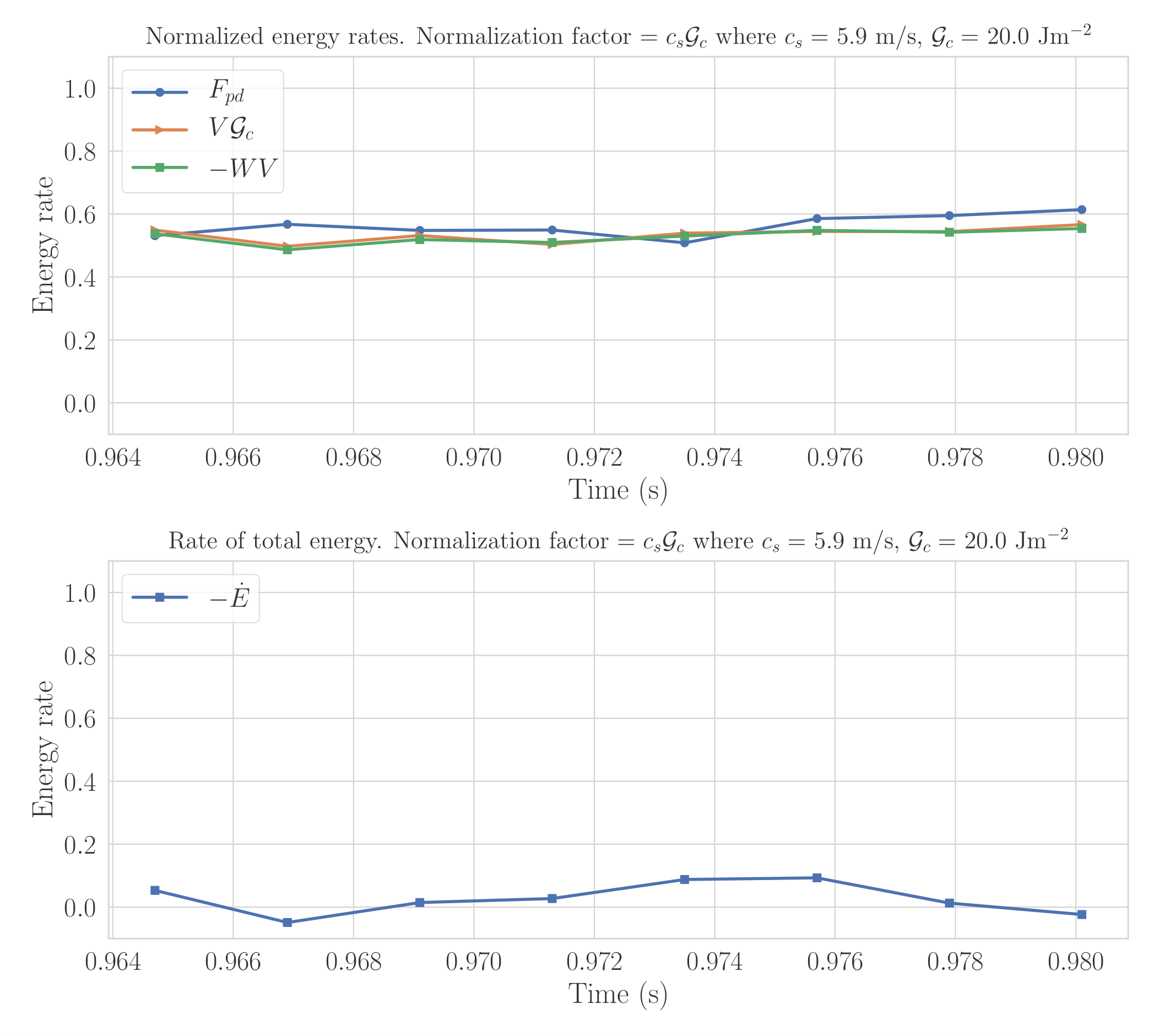
Recent numerical analysis of peridynamic models focus on establishing apriori convergence rates of finite difference and finite element schemes. Initial work on apriori convergence rates for bond and state based peridynamic models have appered in (Jha and Lipton, 2018a), (Jha and Lipton, 2018b),

References

1. L. Ambrosio, A. Coscia, and G. Dal Maso. Fine properties of functions with bounded deformation. Arch. Rational Mech. Anal., 139:201-238, 1997.
2. P.K. Jha and R. Lipton. Numerical analysis of nonlocal fracture models in Holder space. SIAM J. Numer. Anal. 56 (2018a), pp. 906-941.
3. P.K. Jha and R. Lipton. Numerical convergence of nonlinear nonlocal continuum models to local elastodynamics. International Journal of Numerical Methods in Engineering. 114 (2018b), pp. 1389-1410.
4. R. Lipton. Cohesive Dynamics and Brittle Fracture. Journal of Elasticity, 124, Issue 2, 2016, pp. 143-191.
5. R. Lipton. Dynamic Brittle Fracture as a Small Horizon Limit of Peridynamics. Journal of Elasticity, 117, Issue 1, 2014 pp 21-50.
6. S.A. Silling. Reformulation of elasticity theory for discontinuities and long-range forces. Journal of the Mechanics and Physics of Solids, 48:175-209, 2000.