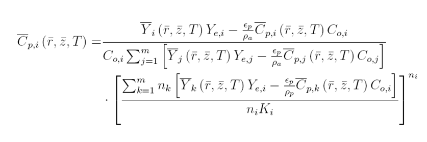
1.3 Non-Linear Coupling Equation
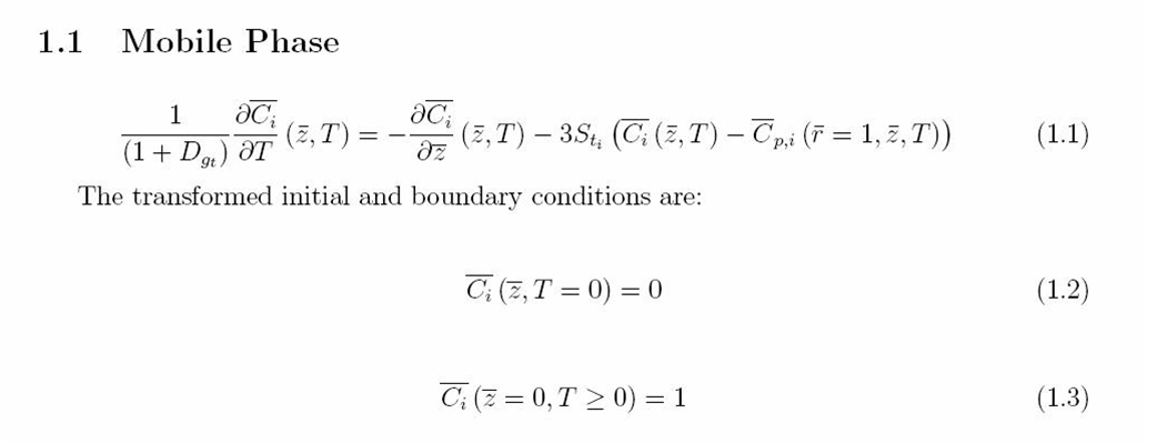
There are three relevant equations used in the development of models for the GAC filter. These three equations model the mobile phase, the pore phase, and the nonlinear coupling equation represents the entirety of the GAC filter. The mobile phase and the pore phase consist of three independent variables being r, z, and T.
R is the radial coordinate, Z is the axial coordinate, T is the time coordinate
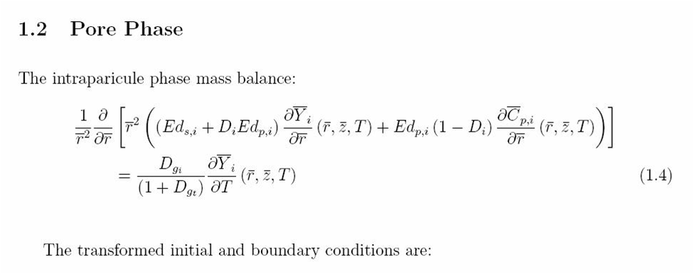
In regards to the pore phase equation we attempted to understand the mathematics behind this equation. It just so happens that the mobile phase model is a symmetric equation with three variables, being the rate of the fluid into the biomass filter, the time at which the particular pore in question is assessed, and the size of the carbon pore in question. We first took the partial derivatives of each of these variables and then we proceeded to plug in the points of our model trials, with these being three, five, and seven grid points. These points are known as collocation points. Once you do this you can arrange each of these solutions together to form three different matrices. This is known as orthogonal collocation. Doing this procedure by hand is very expensive and time consuming, so we have worked together to create a program in Matlab that solves for these matrices for us. However, we still find that it is very crucial to understand the mathematical methods used to determine these matrices. The next step from here will be to further our knowledge of the mobile phase of our model and determine exactly how this phase is deduced mathematically.
In more relevant terms, application of orthogonal collocation is use to solve the relevant equations. This method utilizes Legendre polynomials as trial functions and the collocation points are taken as the root of these Legendre polynomials. The spatial derivatives are expressed in matrix form in terms of the three dependent variables that are evaluated at the collocation points. This process leads to a set of ordinary differential equations where the independent variable is time, T. Then Matlab is utilized to integrate these equations and solve them.
1.3 Non-Linear Coupling Equation