Legendre Roots
The Legendre Roots for the axial points used in the scheme are now calculated using a MATLAB program that auto generates the n th degree Legendre Polynomial. The program uses the generation function described in “Computational Algorithm for Higher Order Legendre Polynomial and Gaussian Quadrature Method” (3) to generate the Legendre polynomials. The roots are then calculated for the symmetric planar geometry and through manipulation of the solutions the correct roots can be produced for symmetric planar geometry, symmetric spherical geometry and non-symmetric planar geometry(used for the axial points). All roots generated are for Legendre Polynomials with a unity weight function. The roots were against verified against “SPEEDUP TM ION EXCHANGE COLUMN MODEL” (1) for the first roots and then against “Multiple Root Finder for Legendre and Chebyshev polynomials via Newton’s Method” (4).
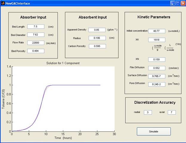
Graphic User Interface
While these accomplishments improve the quality of the simulation most of them can remain hidden from the user of the code so during our time in this project the team also worked to improve on the basic interface to the GAC filter simulation using MATLAB’s built in GUIDE system (4). The new GUI will present the option to change the basic GAC filter properties and approximations without having to manually edit the .m file. The GUI also helps in easily identifying variables and values needed for them as it starts with a default test case already loaded. The new GUI also presents the results incorporated within the interface rather than as a separate graph appearing in a more complete way. The GUI also presents tabs for the selection of different input conditions than constant loading like intermittent loading, input according to a function or input read in from an Excel file. The GUI now also allows printing the results to a Excel file for further analysis.