Some topics in scattering and resonance
Contents
1. Metamaterials: artificial bulk material properties from high-contrast fine structure
- • Artificial magnetism
- • Convergent power series for waves in metamaterials
2. Guided modes in periodic structures and transmission anomalies
- • Modes guided by a periodic slab; Fano resonance in photonic structures.
- • Modes guided by a planar defect in a photonic crystal
3. Calderón boundary-integral projectors
- • Homogeneous media and application to guided modes and scattering
- • Periodic media and application to thick photonic crystal slabs and spectral gaps
4. Boundary-integral numerical code
5. Optimization
- • Manipulation of transmission
- • Density of states for photonic crystal slabs
6. Transmission gaps and anomalies
- • Complete and incomplete spectral gaps
- • Defects and transmission anomalies
- Periodic channel
- Fabry-Perot mirror
- Surface defect
- Random crystals
1. Metamaterials: artificial bulk material properties from high-contrast fine structure
Artificial magnetism
In 1999, John Pendry and others introduced periodic arrays of microresonators as a means of creating magnetism at frequencies for which magnetic response does not occur naturally. The components of the composite are in themselves non-magnetic, and it is the resonance at the fine scale of the resonators that produces magnetic activity. The idea is that the combination of high conductivity and small ratio between the period of the array to the bulk variation of the electromagnetic fields causes a discontinuity in the magnetic field at the edges of the resonators. See the references in [KoSh08], in which we rigorously analyze a 2D model using two-scale homogenization. See also the work of Bouchitté and Schweizer on a 3D model referenced in the same work.
Artificial magnetism can also be created by high-contrast dielectric rods arranged periodically in a neutral host. In the homogeneous limit, a sequence of spectral bands and gaps emerges. See the works of Zhikov, Hempel/Lienau, and Bouchitté/Felbacq referenced in [FLS10ab].
Convergent power series for waves in metamaterials
In formal homogenization of periodically micro-structured media, one expands fields in formal power series with respect to the small cell size. For a finite sample of the composite, one cannot expect the power series to converge to a field in the medium for any non-zero cell size because of boundary effects. But for Bloch waves in infinite high-contrast media, one can prove convergence. This has been done for the two types of meta-material described above in [FSL10b] and [Sh10b]. It even works with a negative material coefficient in the inclusions (the analysis is in fact easier in that case). Thus one actually proves existence of solutions, near but not at the homogenization limit for noncoercive problems!
In certain cases, one can even quantitatively calculate a radius of convergence of these power-series representations of waves and thus obtain a way to compute the fields in specific structures to arbitrary algebraic order of accuracy in the cell-to-wavelength ratio. This analysis was done for plasmonic inclusions (with large negative frequency-dependent index) in the dissertation of Santiago Fortes (Louisiana State University 2009) and in [FLS10a] by using fine properties of the Catalan numbers, which are defined recursively through convolution:
C0 = 1,
Cn+1 = ∑nj=0 Cn-j Cj.
2. Guided modes in periodic structures and transmission anomalies
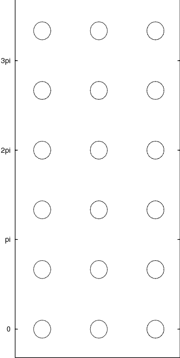
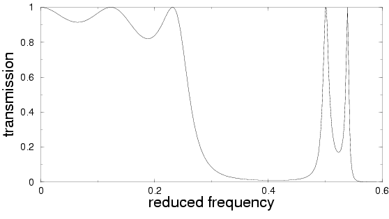
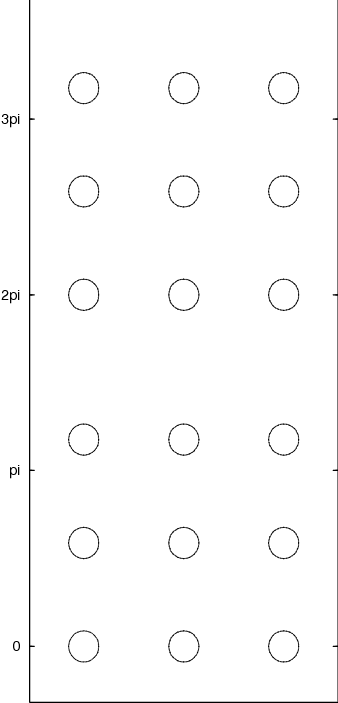
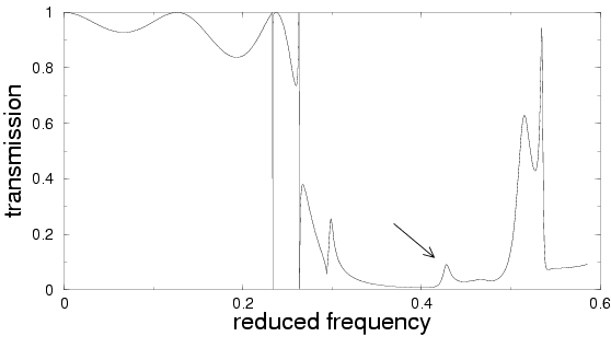
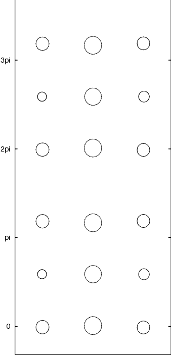
Modes guided by a periodic slab
This is a link to a sequence of
diagrams
and explanations that describes robust and nonrobust guided
modes in slabs of periodic materials surrounded by a homogeneous
medium (as air). It also explains how the nonrobust guided
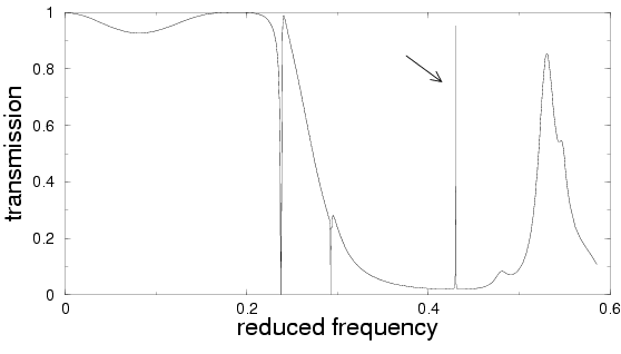
modes give rise to anomalous transmission behavior. A rigorous asymptotic formula generalizes the classical Fano shape. See the
reference [ShVe05] in my list of articles for a study of anomalous
transmission, and see [ShVo07] and Ref. 6 therein (Bonnet-Bendhia/Starling) for the theory of
guided modes in periodic slabs.
Modes guided by a planar defect in a photonic crystal
If we reverse the roles of the periodic structure and the air, then we
have a planar waveguide in a photonic (or acoustic) crystal. Guided
modes may exist in the air at frequencies that are in a spectral
gap for the perfect periodic structure. See Refs. 2
(Ammari/Santosa) and 10 (Kuchment/Ong) in [RaSh08] in my list of
articles. These modes are understood to cause resonant scattering
behavior when a crystal with a planar waveguide, truncated
parallel to the guide, is illuminated by a plane wave. Some simulations of this
resonant scattering behavior are shown in the part of Section 5 of
this page called "Fabry-Perot mirror". Detailed numerical
calculations of resonant transmission spikes are shown in Ref. 15
of [RaSh08].
In [RaSh08], we prove that a spectral gap emerges as an
interval of
zero transmission of energy through a thick slab of a periodic material as
the thickness tends to infinity. We also prove that transmission
anomalies occur at guided mode frequencies for one-dimensional
structures. We employ the Calderón boundary-integral projectors
based on the radiating Green function for the Helmholtz equation
in free space and the decaying Green function for the Helmholtz
equation in a periodic structure.
3. Calderón boundary-integral projectors
The Calderón boundary-integral projectors for elliptic differential
operators are analogous to the Cauchy boundary-integral
projections in the theory of complex variables. There, an
arbitrary function defined on a curve that divides the complex
plane into two domains is
decomposed uniquely into the boundary value of a holomorphic
function on one side of the curve plus the boundary value of
a holomorphic function on the other side, with both functions decaying like 1/z as
z→∞ (unless one of the domains is bounded). These projections are (I ± H), where H is the Hilbert
transform on the boundary, and the identity I arises from the
Sokhotskyi-Plemelj formula.
There is a similar decomposition involving, say, Helmholtz or
Maxwell fields in two domains separated by an interface. The
projections, called the Calderón projectors, involve single- and
double-layer potentials of an appropriate Green function
(analogous to the Cauchy kernel 1/(z-z0). The
choice of the Green function depends on the application. The
reader is referred to Refs. 5 (Costabel/Stephan) and 11
(Nédélec) in [ShVe03] for the projectors for the Helmholtz and
Maxwell equations associated with a bounded scatterer.
Homogeneous media and application to guided modes and scattering
The Calderón projectors provide a natural and beautiful way to
pose the problem of scattering of plane waves by an obstacle.
This could be, say, a bounded obstacle in free space, a bounded
obstacle in a wave-guide, or a periodic slab. In [ShVe03], we
show how to formulate the problem in the case of a periodic
slab and use the properties of the projectors to gain
knowledge about guided modes. The idea of the formulation of
the scattering problem is this: The total field on the boundary
of the scatterer together with its normal derivative (its trace) have values coming from the interior of the
scatterer and values coming from the exterior, and these value must be matched
appropriately. Both interior and exterior traces are decomposed into traces of the source and
scattered fields. In the
interior, this decomposition coincides with the decomposition
arising from the
complementary Calderón projectors constructed from a
Green function with the interior material properties, and in the
exterior, it coincides with the decomposition arising from the
projectors that use the radiating Green function with the
exterior material properties. Projecting onto the traces of the
(known) source fields in the exterior and interior gives an
equation of the form (B + C)u = f, where B is bounded, C is
compact, u is the trace of the total field, and f is essentially
the trace of the sum of the source fields.
Seeing that B and C depend analytically on the frequency ω and the
Bloch wave vector κ parallel to the slab, the equation (B + C)u =
0 gives rise to a complex dispersion relation between κ and ω
corresponding to generalized guided modes of the slab.
Real-valued pairs (κ,ω) correspond to true guided modes. Since
the imaginary part of ω on the dispersion relation must be
negative, typical pairs correspond to fields that are decaying
in time but exponentially growing spatially with distance from
the slab. These are analogous to the fields of the "scattering
resonances" for the Helmholtz resonator; see Ref. 6
(J. T. Beale) of [ShVe03].
Periodic media and application to thick photonic crystal slabs and spectral gaps
In [RaSh08], we extend the Calderón projectors to
interfaces between two complementary subdomains of a periodic
medium. We then use these to investigate the limiting behavior of transmission of
harmonic fields at frequencies in a spectral gap of the medium.
4. Boundary-integral numerical code
For the simulations of fields in periodic slabs that you see on this page, we used a numerical code developed at
Duke University by M. Haider, S. Shipman, and S. Venakides
[HaShVe02]. It is based on the integral representations
that are formulated most elegantly using the Calderón
boundary-integral projectors mentioned above [ShVe03].
The algorithm uses an acceleration technique that is similar to a
multipole algorithm, specialized to periodic structures. Most
efficiency is gained when the number of periods across the slab is very large.
References on multipole algorithms can be found on the website of
L. Greengard.
5. Optimization
Manipulation of transmission
In [LiShVe03], we develop the variational calculus for the
transmission coefficient as a function of the material parameters
ε and μ for two-dimensional scattering of electromagnetic plane
waves by periodic slabs. The Lp theory of the variational calculus is made rigorous in [Sh08]. The simulations below show how
transmission features can be optimized with the resulting
gradient-flow algorithm.
Perfect square lattice with no channel
Perfect square lattice with a channel every three rows
Perturbed lattice with channels
Intensity of the scattered field at the frequency of the peak
transmission above

Moving a transmission gap
Density of states for PC slabs
I have implemented an algorithm for optimizing
the "effective density of states" for a photonic crystal slab.
This effective density is discussed in
[Bendickson/Dowling/Scalora, Phys. Rev. E, 53 No. 4 p. 4107].
It is essentially the sensitivity of the effective wave number
of a scattered field across the slab with respect to frequency
and is thus directly related to the phase of the complex
transmission coefficient. Anomalous behavior of this quantity
coincides with resonant scattering in the structure and
anomalous transmission of energy (the magnitude of the
transmission coefficient).
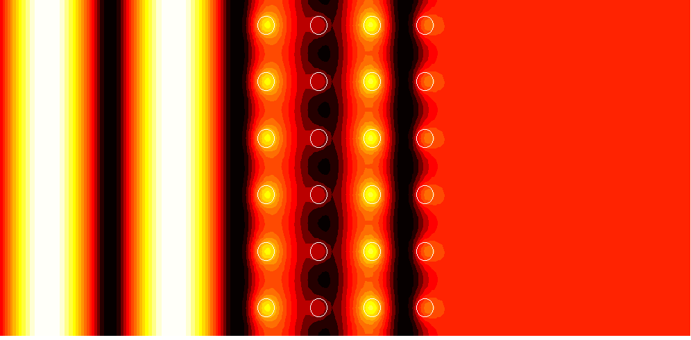
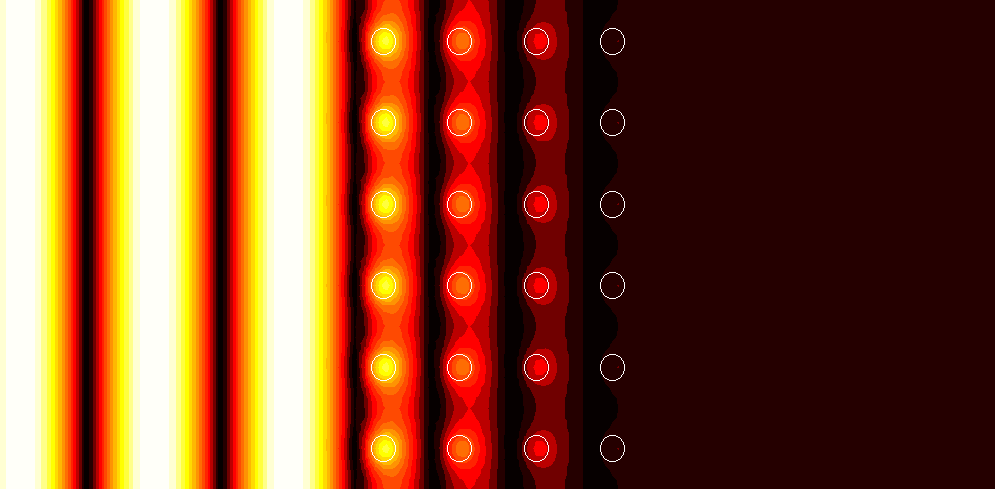
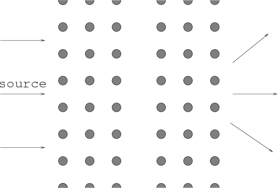
6. Transmission gaps and resonant transmission: Simulations
Below are some simulations of resonant scattering and
transmission behavior. They show electrically polarized fields in
two-dimensional structures that are periodic in one direction and
finite (truncated) in the other. The dielectric constant ε is taken to be
around 10 to 12, and the magnetic constant is taken to be 1.
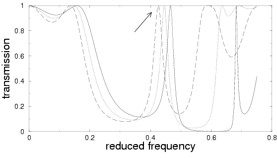
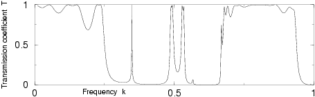
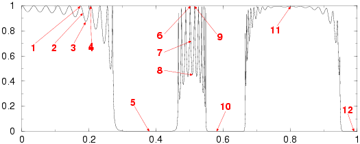
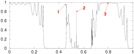
Complete and incomplete spectral gaps
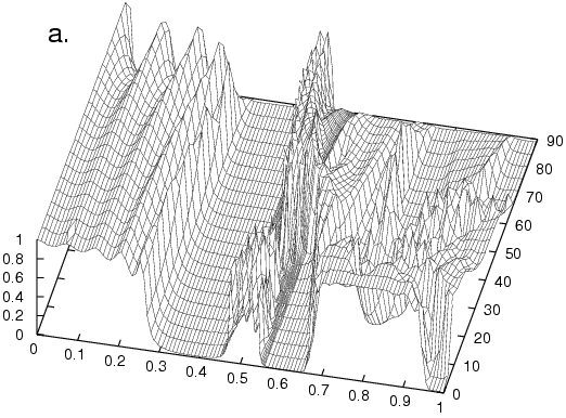
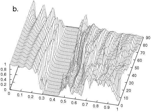
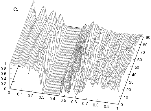
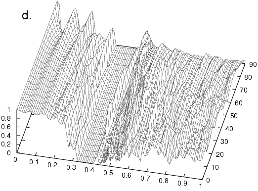
Graph (a) below shows the transmission of energy through an infinite slab of a
square-lattice photonic crystal of circular rods, five rods
thick, as a function of reduced frequency (from 0 to 1) and
angle of incidence (from 0° to 90°).
Notice the complete
gap from frequencies of about 0.3 to 0.45 and the
incomplete gap around 0.6. Graphs (b), (c), and (d)
show realizations of how the transmission changes under random perturbations of
the centers of the five rods in a period (the structure
remains periodic---the perturbations are the same in each
period). In (b), the perturbations are taken to uniformly
distributed up to 10% of the distance between adjacent rods, in
(c), it is 20% and in (d) it is 30%.
Observe that the complete
gap is robust under these perturbations, whereas the
incomplete gap is not.
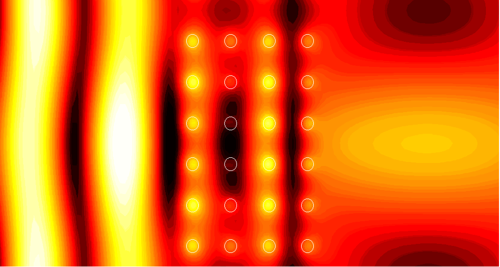
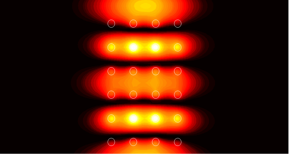
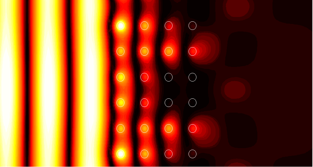
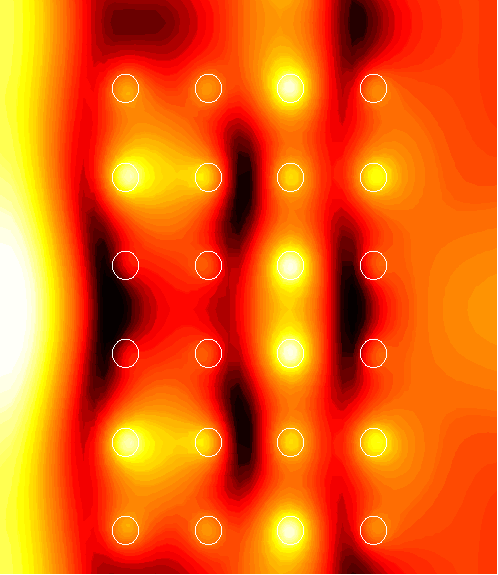
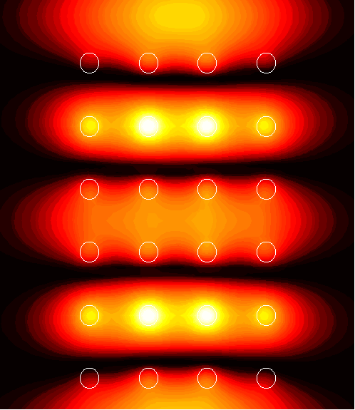
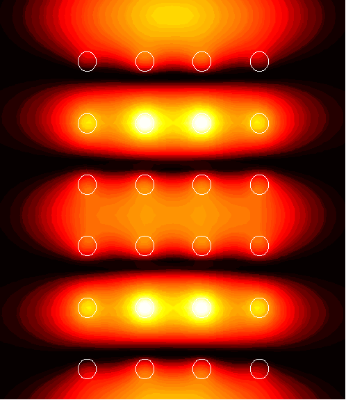
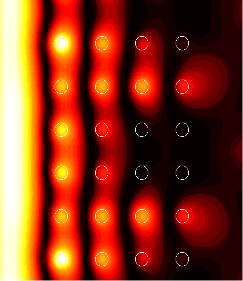
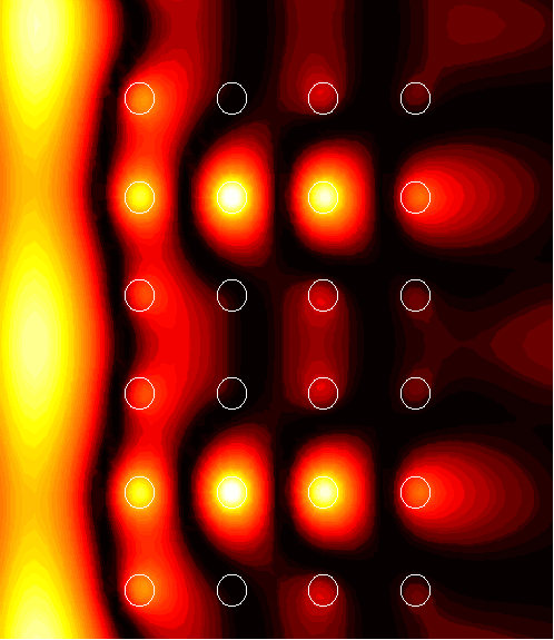
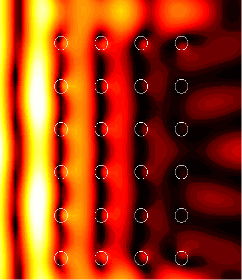
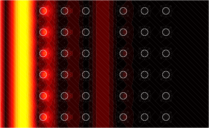
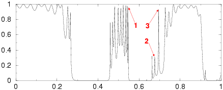
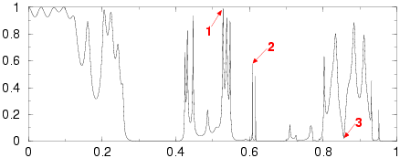
Defects and transmission anomalies
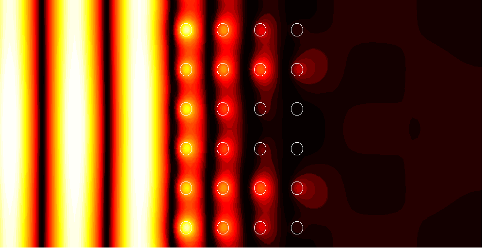
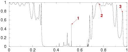
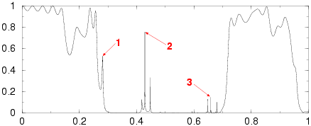
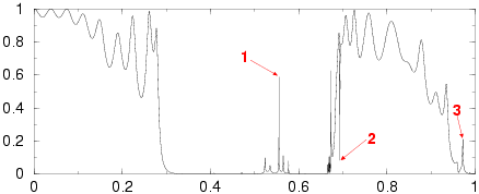
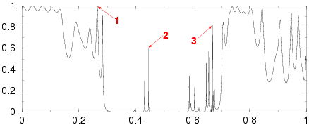
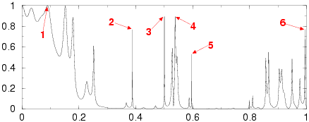
Defects in an otherwise perfect structure cause resonance, resulting in amplitude enhancement in the structure and transmission anomalies. The simulations show the amplitude of an electrically polarized field scattered by the structure; the numbers above the images indicate the maximum amplitude enhancement.
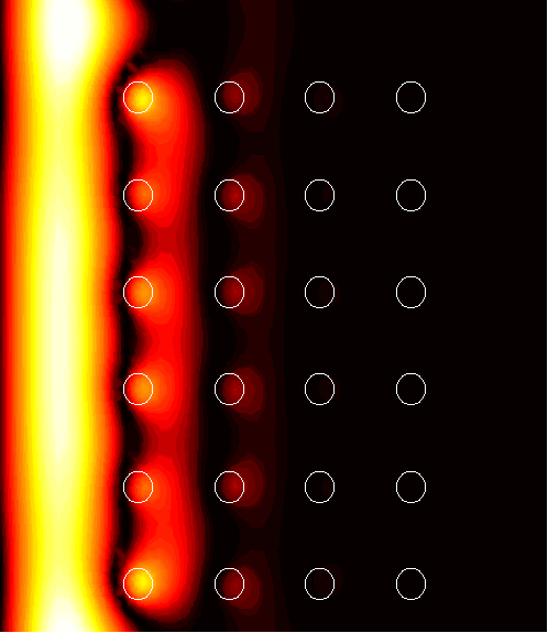
Periodic channel
Perfect 6x4 supercell
1. (1.54)
|
2. (1.99)
|
6x4 supercell with a channel of width d=0.25 relative to the period after each 6 rows (seen in the images at the top of the supercell)
1. (1.62)
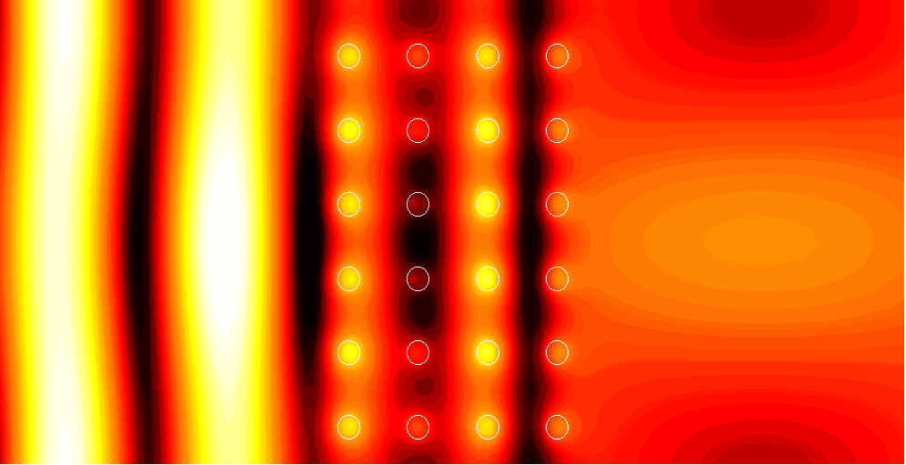
|
2. (137.1)
|
3. (2.05)
|
4. (2.77)
|
6x4 supercell with a channel of width d=0.5
1. (1.67)
|
2. (108.2)
|
3. (2.10)
|
4. (3.70)
|
6x4 supercell with a channel of width d=0.5
1. (1.54)

|
2. (1.76)
|
3. (108.2)
|
4. (61.2)
|
5. (2.09)
|
6. (2.67)
|
7. (10.5)
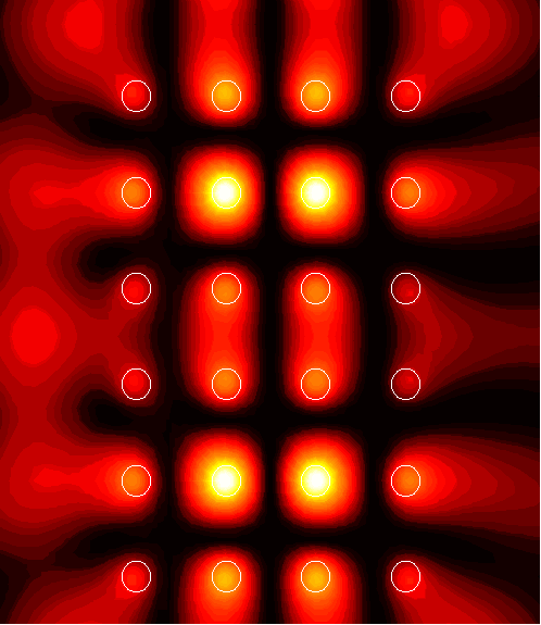
|
8. (2.26)
|
9. (3.70)
|
10. (2.24)
|
11. (2.23)
|
12. (2.22)
|
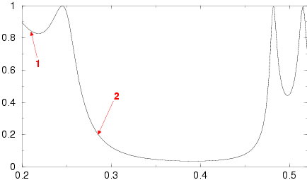
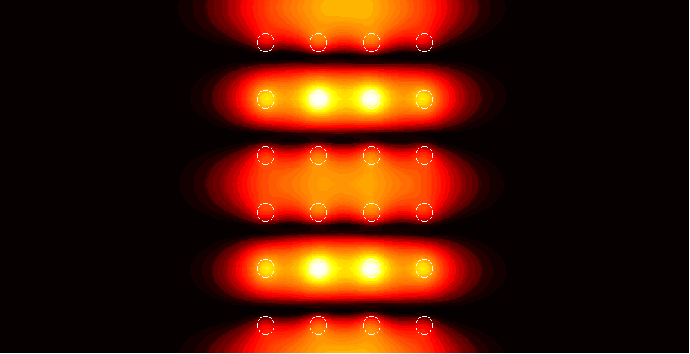
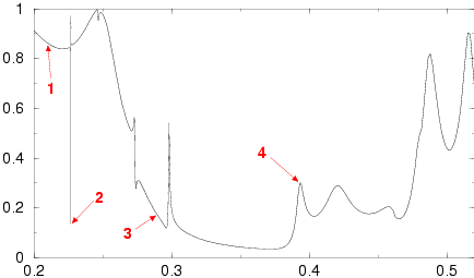
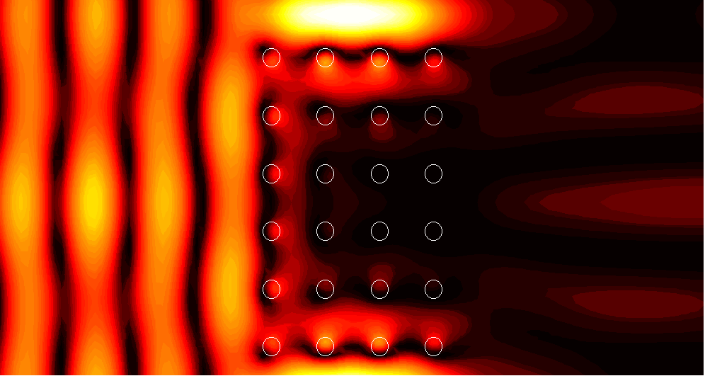
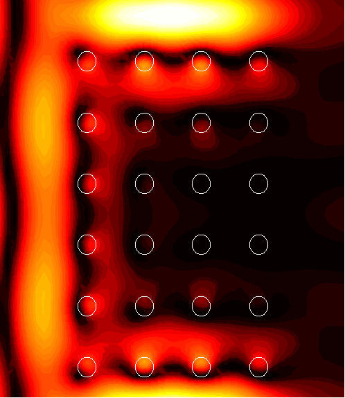
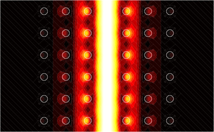
Fabry-Perot mirror
Scattering by a Fabry-Perot photonic crystal mirror.
Transmission through a Fabry-Perot photonic crystal mirror.
Field intensity at a typical frequency in the gap and at a resonant
frequency corresponding to a transmission spike.
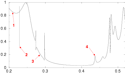
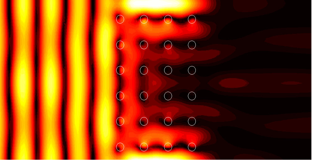
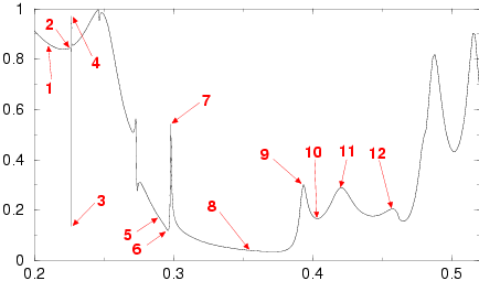
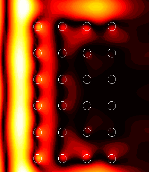
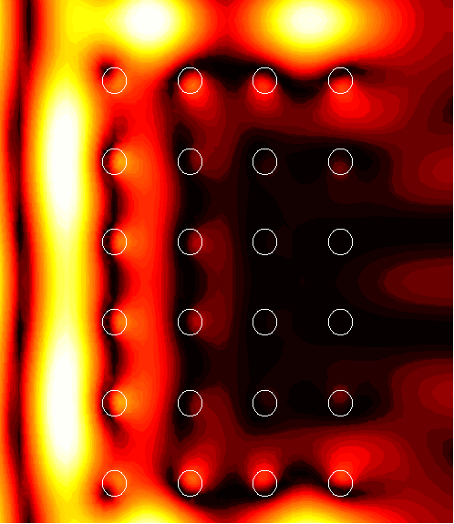
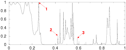
Surface defect
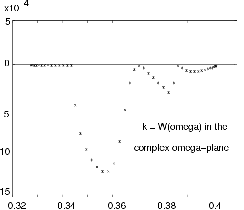
The complex dispersion relation w=W(k) for real values of the wave vector
from 0.401=W(0.0) to 0.327=W(0.5). There are evidently three points with
Re(W(k))=0, corresponding to nonrobust guided modes and a
dispersion relation starting at k=0.344 for robust guided modes.
A nonrobust guided mode at k=0.0, w=0.401.

A robust guided mode at k=0.50, w=0.327.

Scattered field at k=0.0, w=0.271.

Scattered field at k=0.23, w=0.368, near a nonrobust guided mode.

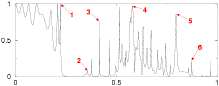
Random crystals
The numbers in parentheses refer to the ratio of the maximal
intensity of the field compared to the intensity of the
incident field.
Perfect 1x10 supercell
1. (1.12)

2. (1.32)

3. (1.48)

4. (1.47)

5. (2.01)

6. (4.17)

7. (3.00)

8. (1.96)

9. (4.48)

10. (2.16)

11. (2.17)

12. (2.70)

1x10 supercell with 10% random perturbations of centers
1. (9.80)

2. (43.84)

3. (2.16)

1x10 supercell with 20% random perturbations of centers
1. (25.85)

2. (2.51)

3. (5.40)

1x10 supercell with 20% random perturbations of centers
1. (7.91)

2. (35.88)

3. (40.49)

1x10 supercell with 30% random perturbations of centers
1. (36.17)

2. (14.59)

3. (8.43)

1x10 supercell with 30% random perturbations of centers
1. (3.42)

2. (57.62)

3. (16.04)
1x10 supercell with 10% random perturbations of radii
1. (12.66)

2. (14.09)

3. (11.07)

1x10 supercell with 30% random perturbations of radii
1. (7.26)

2. (23.26)

3. (4.99)

1x10 supercell with 30% random perturbations of radii
1. (5.52)

2. (2.43)

3. (5.52)

1x10 supercell with 50% random perturbations of radii
1. (4.62)

2. (2.00)

3. (3.32)

4. (21.05)

5. (6.06)

6. (9.91)

1x10 supercell with 50% random perturbations of radii
1. (1.23)

2. (25.23)

3. (25.61)

4. (5.53)

5. (31.62)

6. (25.82)

5x5 supercell, 30% random perturbations of centers,
30° angle of incidence
(11.03)
|