Fall 2013 Capstone Projects
Rain CII Carbon Project
Group 3
Description
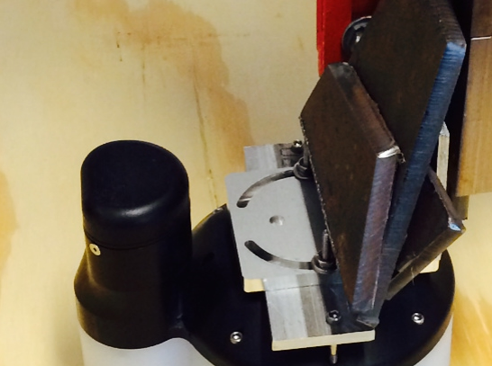
Our group was given a task of creating a mathematical model, implementing a program, and correcting errors using data produced by a robot or “puck”. The puck is used to scan objects for imperfections. The puck's transceiver scans the object while its eight sensors relay information in the form of an $x$ and $y$ component. The model was supposed to use the given data and produce a mapping of where the puck moved. More precisely, we wanted to plot where the transceiver on the puck had moved and correct errors in the plot. We created two models. Both of these models were produced in Matlab.
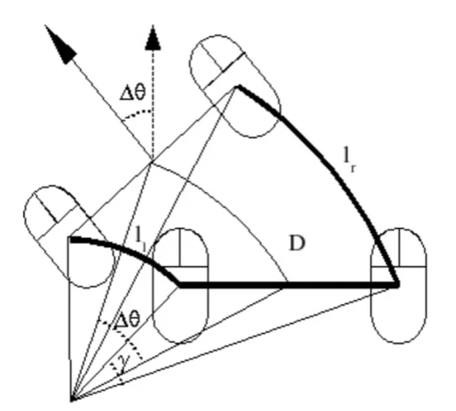
One model, Pose, was based on a paper written by Bonarini, and the other model uses a recurrence relation to plot each sensor's path. We ran into problems with Pose, because the data we were given contained a large amount of zeros which the program couldn't handle. We corrected this by making all the zeros equal a tiny sum. We, then, encountered more problems with other equations because of zeros showing up in the denominators. We corrected these problems, but almost all the images produced weren't showing the results we wanted.
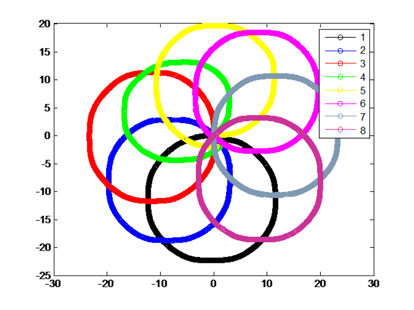
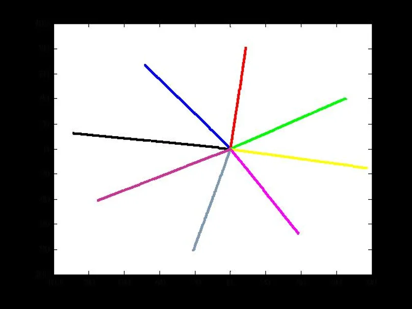
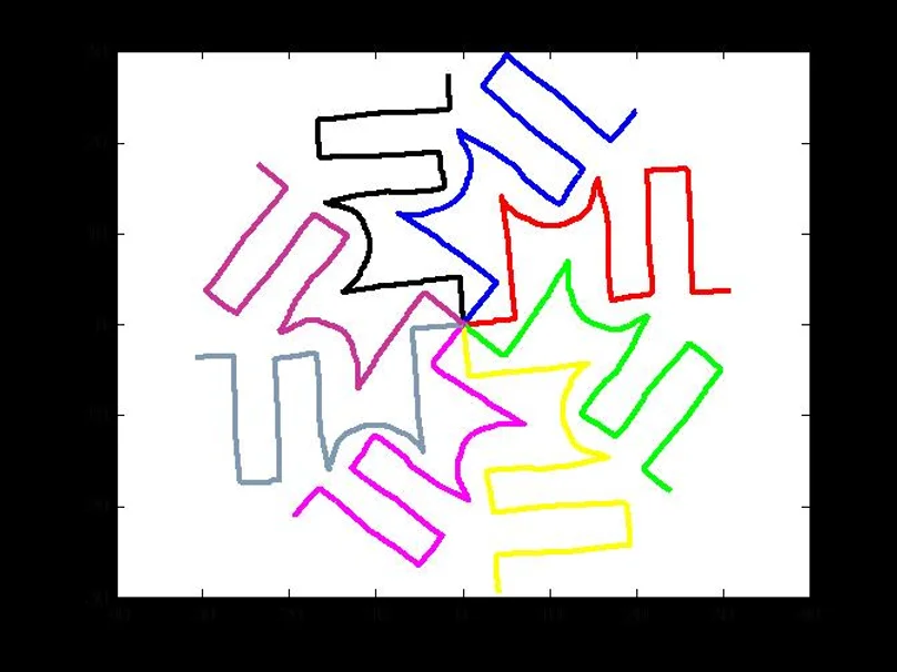
The second model we created was able to map the puck's movements without running into any problems associated with Pose. The resulting images, which are shown in the results page, accurately showed the path of each sensor. We, also, were able to measure the length of path of each sensor. This allowed us to see which path was shortest and therefore contained the most errors.
Programs
Pose model based on Bonarini paper
clear all
clc
numData=xlsread('Results-test1.xlsx','H5:W8386');
% numData=xlsread('Results-test1.xlsx','H8918:W8947');
% numData=xlsread('Results-test1.xlsx','H8586:W90366');
% numData=xlsread('Results-test1.xlsx','H5:W9186');
numData=xlsread('best - TEST_LABCIRCLE _ 011.xlsx','H5:W1003');
% numData=xlsread('TEST_Evisive 6_ 008-60ipm.xlsx','H5:W2220');
% numData=xlsread('TEST_Evisive 6_ 012-120ipm.xlsx','H5:W2340');

E=1.0/1600
x1=-numData(:,1)*E;
y1=numData(:,2)*E;
x2=numData(:,9)*E;
y2=-numData(:,10)*E;

E=.00001
for i= 1:length(x1)
    if (x1 (i)~=0)
    E=E;
    else
      x1(i)=E;
    end
end
for i= 1:length(y1)
    if (y1 (i)~=0)
    E=E;
    else
      y1(i)=E;
    end
end
for i= 1:length(x2)
    if (x2 (i)~=0)
    E=E;
    else
      x2(i)=E;
    end
end
for i= 1:length(y2)
    if (y2 (i)~=0)
    E=E;
    else
      y2(i)=E;
    end
end
l1=sqrt(x1.^2+y1.^2);
l2=sqrt(x2.^2+y2.^2);
xc(1)=0.
yc(1)=0.
thetac(1)=0.
% the position and the direction of the robot at time t
% plot(x1,y1,x2,y2)
cc=[ x1 y1 x2  y2];
% figure(1)
% plot(x1,y1)
% figure(2)
% plot(x2,y2)
s=length(x1)
t=length(y1)
% alpha1=zeros(s)
% alpha2=zeros(s,t);
% alpha1=acos(x1/l1);
% alpha2=acos(y1/l1);
% c=[ alpha1 alpha2]
% alpha(1)=acos(x1 (1)/l1(1));
alpha1(1)=acos(x1 (1)/l1(1));
alpha2(1)=acos(x2 (1)/l2(1));

for i= 2:length(x1)
    if (l1 (i)~=0)
        alpha1(i)=acos(x1 (i)/l1(i));
    else
        alpha1(i)=alpha1(i-1);
    end
end

alpha2(1)=acos(x2 (1)/l2(1))

for i= 2:length(x1)
    if (l2 (i)~=0)
        alpha2(i)=acos(x2 (i)/l2(i));
    else
        alpha2(i)=alpha2(i-1);
    end
end

ss1=alpha1';
ss2=alpha2';
D=1.62
gamma=abs(alpha1-alpha2);

gamma=gamma';
dtetha=sqrt (l1.^2+l2.^2-2*cos (gamma).*l1.*l2).*sign (y2-y1)/D;
dtethavvv=sqrt(l1 (5)^2+l2 (5)^2-2*cos(gamma(5))*l1(5)*l2(5))
r1(1)=0;
r2(1)=0;
for i= 2:length(x1)
    if (dtetha (i)~=0)

        r1(i)=l1 (i)/abs(dtetha(i));
        r2(i)=l2 (i)/abs(dtetha(i));
        % alpha2(i)=acos(y1 (i)/l1(i));
    else
        alpha1(i)=alpha1(i-1);
        r1(i)=r1(i-1);
        r2(i)=r2(i-1);
       % alpha2(i)=alpha2(i-1);
    end
end

r1=r1';
r2=r2';

sst=[ss1 ss2 gamma dtetha r1  r2 ];
xp2=r2.*(sin(ss2+dtetha)-sin(ss2)).*sign(dtetha)+D/2;
yp2=r2.*(cos(ss2)-cos(ss2+dtetha)).*sign(dtetha);
xp1=r1.*(sin(ss1+dtetha)-sin(ss1)).*sign(dtetha)-D/2;
yp1=r1.*(cos(ss1)-cos(ss1+dtetha)).*sign(dtetha);
cc2=[xp1 yp1  xp2  yp2];
deltax=(xp1+xp2)/2;
deltay=(yp1+yp2)/2;
 dtetha1(1)=0

for i= 2:length(x1)
    if (deltax (i)~=0)
        dtetha1(i)=atan(deltay (i)/deltax(i));
    else
        dtetha1(i)=dtetha1(i-1);
    end
end
 dtetha1= dtetha1'

xc(1)=0.;
yc(1)=0.;
thetac(1)=0.;

for i= 2:length(x1)
    xc(i)=xc(i-1)+sqrt(deltax (i-1)^2+deltay (i-1)^2)*cos(thetac(i-1)+dtetha1(i-1));
    yc(i)=yc(i-1)+sqrt(deltax (i-1)^2+deltay (i-1)^2)*sin(thetac(i-1)+dtetha1(i-1));
    thetac(i)=thetac(i-1)+dtetha(i-1);
end

cc1=[ xc' yc' thetac']
figure(3)
plot(xc',yc')
Second model
clear all
clc
numData=xlsread('Results-test1.xlsx','H5:W9186');
% numData=xlsread('TEST_LABCIRCLE _ 001.xlsx','H5:W3193');
% numData=xlsread('TEST_Evisive 6_ 008-60ipm.xlsx','H5:W4220');
numData=xlsread('TEST_Evisive 6_ 012-120ipm.xlsx','H5:W2340');
% numData=xlsread('best - TEST_LABCIRCLE _ 011.xlsx','H5:W1075');
numData=xlsread('best - TEST_LABCIRCLE _ 011(2).xlsx','H5:W1075');

theta=pi/2
H1=cos(theta)
H2=sin(theta)
C = {'k','b','r','g','y','m',[.5 .6 .7],[.8 .2 .6]} % Cell array of colros.
    m=1
for k=1:8

x1=numData (:,m)/1600;
y1=numData (:,m+1)/1600;
% x2=numData (:,3)/1600;
% y2=numData (:,4)/1600;
E=0.00001;
D=1.62/2;
N=1000;
 xc1(1)=x1(1);
 yc1(1)=y1(1);
  % xc2(1)=x2(1)
% yc2(1)=y2(1)
for i= 2:length(x1)
    xc1(i)=xc1(i-1)+x1(i);
    yc1(i)=yc1(i-1)+y1(i);
   % xc2(i)=xc2(i-1)+x2(i);
    % yc2(i)=yc2(i-1)+y2(i);
end
sss=k
% hold all
figure(1)
% axis square
% title('sensor ')

subplot(4,2,k);

% plot(xc1',yc1')
plot(xc1',yc1','color',C{k},'LineWidth',2)
% radius=sqrt ((yc1(length(x1))-yc1(1))^2+(xc1(length(x1))-xc1(1))^2)/(2*pi)
title(sprintf('sensor %2 .0f ',sss))
% title(sprintf('radius %3 .0f ',radius))
m=m+2
end

x1=numData (:,13)/1600;
y1=numData (:,14)/1600;
x2=numData (:,1)/1600;
y2=numData (:,2)/1600;
% figure(4)
% plot(y1,y2)

xc1(1)=x1(1);
yc1(1)=y1(1);
xc2(1)=x2(1);
yc2(1)=y2(1);

 for i= 2:length(x1)
    xc1(i)=xc1(i-1)+x1(i);
    yc1(i)=yc1(i-1)+y1(i);
    xc2(i)=xc2(i-1)+x2(i);
    yc2(i)=yc2(i-1)+y2(i);
end
figure(2)

% plot(xc1',yc1',-xc2',-yc2','LineWidth',2)
% plot(xc1',yc1',-yc2',xc2')% sensor 1
plot(xc1',yc1',(xc2'*H1-yc2'*H2),(xc2'*H2+yc2'*H1),'LineWidth',2)
m=1
C = {'k','b','r','g','y','m',[.5 .6 .7],[.8 .2 .6]} % Cell array of colros.
    for k=1:8

x1=numData (:,m)/1600;
y1=numData (:,m+1)/1600;
% x2=numData (:,3)/1600;
% y2=numData (:,4)/1600;
E=0.00001;
D=1.62;
N=1000;
 xc1(1)=x1(1);
 yc1(1)=y1(1);
  % xc2(1)=x2(1)
% yc2(1)=y2(1)
for i= 2:length(x1)
    xc1(i)=xc1(i-1)+x1(i);
    yc1(i)=yc1(i-1)+y1(i);
   % xc2(i)=xc2(i-1)+x2(i);
    % yc2(i)=yc2(i-1)+y2(i);
end
sss=k
hold on
figure(3)
% axis square
% title('sensor ')
plot(xc1',yc1','color',C{k},'LineWidth',2)
% plot(xc1',yc1')
% legend(num2str((k)))
legend({'1';'2';'3';'4';'5';'6';'7';'8'})

m=m+2
end
n=1
theta=0
for k=1:8

H1=cos(theta)
H2=sin(theta)
x1=numData (:,n)/1600;
y1=numData (:,n+1)/1600;
% x2=numData (:,3)/1600;
% y2=numData (:,4)/1600;
E=0.00001;
D=1.62;
N=1000;
 xc1(1)=x1(1);
 yc1(1)=y1(1);
  % xc2(1)=x2(1)
% yc2(1)=y2(1)
for i= 2:length(x1)
    xc1(i)=xc1(i-1)+x1(i);
    yc1(i)=yc1(i-1)+y1(i);
   % xc2(i)=xc2(i-1)+x2(i);
    % yc2(i)=yc2(i-1)+y2(i);
end
sss=k
hold on
figure(6)
% axis square
% title('sensor ')%%%%%%%%%%%%%%%%%%%%%%%%%%%%%%%%%%%%%%%%%%%%%%%%%%%%%%%%%%
% plot(xc1',yc1','color',C{k},'LineWidth',2)
plot((xc1'*H1-yc1'*H2),(xc1'*H2+yc1'*H1),'color',C{k},'LineWidth',2)
%%%%%%%%%%%%%%%%%%%%%%%%%%%%%%%%%%%%%%%%%%%%%%%%%%%%%%%%%%%%%%%%%%%%%%%%%%
% plot(xc1',yc1')
% legend(num2str((k)))
legend({'1';'2';'3';'4';'5';'6';'7';'8'})

n=n+2
theta=theta+pi/4

end
Data/Results
Our report is attached to this webpage.
Data was collected which represents distinct ways of moving the robot. Using the given data which contained the change in $x$ and the change in $y$ of 8 individual sensors, the two programs produced graphs that mapped each sensor's movement.
Evisive Visit
This is a video taken on a field trip to Evisive, the company our project is under. In the picture an actual scan using the puck is shown. An image of the scan produced by our second model can be seen in the data/results section of this page.
Final presentation
This video shows our final power point presentation.
| Attachment | Size |
|---|---|
| 20.92 KB |